The transition from manual calculation to automated computing began with 19th-century mechanical designs and culminated in mid-20th-century electro-mechanical systems.
Era 0: Pre-mechanical calculation and early automata (Antiquity–1830s)
Computing has evolved along two parallel paths:
Foundational calculation tools
Before mechanical gears were introduced, human calculation was heavily bottlenecked by working memory, specifically the cognitive load of tracking intermediate sums, carrying tens, and executing multi-step multiplication. Early tools were designed not to automate thought, but to serve as external, physical registers and lookup systems.
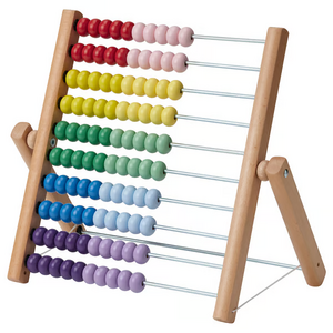
The Abacus (c. 2700–500 BCE) — Positional memory register
How it works: Rather than calculating on its own, an abacus acts as an external physical register. Beads arranged on parallel rods or grooves represent specific decimal place values (units, tens, hundreds, thousands).
Cognitive relief: The user executes mental arithmetic rules, but never needs to hold multi-digit numbers or carries in short-term memory; the physical position of the pushed beads instantly stores the current state and intermediate results.
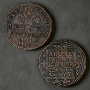
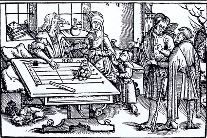
The counting board and jetons (Medieval to renaissance Europe, c. 1100–1600s) - Positional grid computation
How it works: Rather than beads permanently fixed on wires, European merchants and money-changers used a flat wooden table or cloth marked with parallel lines representing powers of ten (or British pounds, shillings, and pence). Calculations were performed by physically placing, sliding, and clearing metal cast counters called jetons.
Cognitive relief: It allowed rapid commercial accounting in Roman-numeral Europe without requiring written scratch paper. By turning complex currency conversions into physical movement of tokens across labeled lines, the clerk avoided mental carrying mistakes.counting board and jetonsboard and jetons table
Historical context: Why physical aids preceded pen-and-paper calculation
While performing arithmetic with pen, paper, and written digits seems fundamental today, dynamic calculation using scratch paper was impractical for most of human history due to economic, linguistic, and cognitive barriers:
Scarcity and cost of writing media: Prior to industrial wood-pulp papermaking in the 19th century, writing surfaces such as papyrus, vellum (animal skin), and rag paper were costly commodities reserved for legal deeds, state censuses, and holy texts. Wasting consumable sheets on intermediate scratch work and discarded calculations was financially prohibitive. Physical instruments like the abacus, counting boards, or sliding rules could be reset indefinitely without consuming materials.
Limitations of pre-positional numeral systems: Western commerce historically operated under Roman numerals (I, V, X, L, C, D, M), which lacked a zero and place-value notation. Attempting to perform multi-digit multiplication or long division symbolically on paper using Roman numerals is exceptionally difficult. As a result, computation was handled externally on physical lines (using stones or tokens called jetons), and paper was used exclusively at the very end to record the final sum.
High barrier of mathematical literacy: Even after the Hindu-Arabic positional decimal system was popularized in Europe via Fibonacci's Liber Abaci (1202), written algorithmic arithmetic ("algorism") remained an elite academic skill taught in specialized guild schools. Tactile counting frames allowed merchants and apprentices to compute rapidly through physical rules without needing advanced arithmetic literacy.
Human working memory and error propagation: Long multi-digit manual arithmetic forces the human brain to simultaneously recall multiplication tables, track running carry values, and transcribe staggered sums—each step introducing points of human failure. Physical tools effectively externalized cognitive registers:
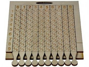
Napier's Bones physically encoded the multiplication table, converting multi-digit operations into simple diagonal single-digit additions.
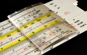
The Slide Rule converted algebraic multiplication and division into continuous spatial distances, allowing an engineer to obtain multi-digit approximations in seconds without performing a single written calculation.
Functional division: Pen-and-paper vs. physical calculation aids
Factor
Pen-and-Paper Arithmetic
Physical Calculation Aids
Resource model
Consumable (ink, parchment, or rag paper spent per calculation)
Advanced numeracy, literacy, and memorized carrying algorithms
Simple tactile motion rules; functional across different languages/scripts
Primary historical role
Static storage: Preserving final results, deeds, and ledgers
Dynamic processing: Real-time arithmetic and intermediate state tracking
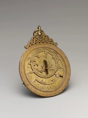
The Astrolabe (c. 400–1500s) - Two-dimensional analog celestial calculator
How it works: Highly refined by Islamic Golden Age astronomers and mathematicians, the planispheric astrolabe mapped the 3D celestial sphere onto a flat, rotating brass coordinate plate (stereographic projection).
Cognitive relief: Instead of solving complex spherical trigonometry formulas by hand, navigators and astronomers could solve local solar time, twilight, prayer hours, and planetary positions in seconds by aligning sighting pointers on the brass plate with the observed altitude of a star or the sun.Astrolabio
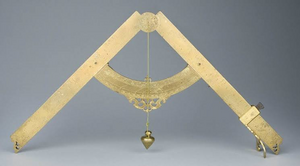
The Sector or Proportional Compass (c. 1560) - Geometrical proportional calculator
How it works: Developed independently by inventors such as Fabrizio Mordente, Guidobaldo del Monte, and perfected by Galileo Galilei, the sector consisted of two hinged brass arms marked with calibrated scales (arithmetic, geometric, trigonometric).
Cognitive relief: Using the geometric theorem of similar triangles and a simple pair of dividers, operators could calculate proportions, scale drawings, compute gunnery trajectories, and extract square or cube roots mechanically without performing manual long-hand arithmetic.Proportional compass
Napier’s Bones (1617) - Lattice multiplication on rods
How it works: Invented by Scottish mathematician John Napier, this tool consists of a set of indexed wooden, bone, or ivory rods inscribed with multiplication tables. Each square on a rod is divided by a diagonal line separating tens from units (the basis of lattice or "gelosia" multiplication).
Cognitive relief: To multiply a complex number (e.g., 425 × 7), the operator simply arranges the rods labeled 4, 2, and 5 side by side. Reading across row 7, the multiplication is instantly converted into simple, low-effort diagonal additions of adjacent digits, completely eliminating the need to memorize or look up multiplication tables.
The Slide Rule (1622) — Logarithmic analog computation:
How it works: Developed by William Oughtred and others shortly after Napier defined mathematical logarithms, the slide rule places logarithmic scales onto sliding linear rules.
Cognitive relief: Because logarithms translate multiplication into addition (log(a · b) = log a + log b) and division into subtraction, a user can multiply or divide two numbers simply by aligning sliding physical distances. The operator offloads difficult calculation to a fast, visual spatial alignment, yielding results accurate to three or four significant digits.slide rule oughtred
Mechanical calculating machines
designed to automate calendar cycles, astronomical tracking, and arithmetic carry operations.
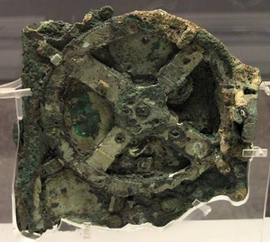
Antikythera mechanism (c. 150–100 BCE): An ancient Greek bronze mechanism comprising over 30 intricate differential gears. Used to track and predict lunar phases, solar cycles, Olympiads, and eclipses, it represents the earliest known geared analog computing device.antikythera
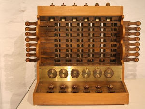
Schickard's calculating clock (1623): German polymath Wilhelm Schickard designed the earliest documented mechanical calculator using linked gear wheels and single-tooth trip mechanisms to automate multi-digit addition and subtraction.schickards calculating clockhttps://www.youtube.com/shorts/vi_33gmJoBU
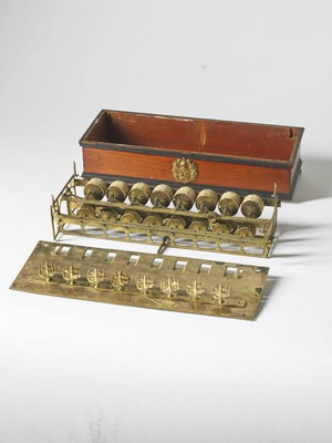
Pascal's Pascaline (1642): Built by Blaise Pascal to aid his father in taxation records, the Pascaline became the first widely recognized, operational mechanical adder. Its central breakthrough was the sautoir, a gravity-weighted pawl mechanism that reliably handled multi-dial tens carry operations.Pascal's pascaline
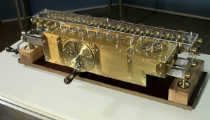
Leibniz's Stepped Reckoner (1673): Gottfried Wilhelm Leibniz introduced the stepped gear cylinder (the Leibniz wheel), enabling a mechanical machine to perform direct multiplication and division alongside addition and subtraction. Leibniz was also the first to systematically document the modern binary number system (1679).Leibniz reckoner
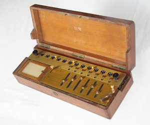
Thomas de Colmar's Arithmometer (1820): The first mechanically reliable, commercially manufactured calculator capable of daily office use, bringing four-function desktop calculation into mass adoption across finance and engineering.Colmar arithmometer
The Jacquard Loom (1804): The dawn of stored instruction In 1804, French weaver Joseph Marie Jacquard revolutionized textile production by automating loom operations through punched card chains. Perforated holes in stiff cards mechanically determined whether individual warp threads were lifted or lowered. While not designed for mathematical computation, Jacquard’s invention demonstrated the principle of external programmability, the ability to change the machine's task dynamically by feeding it a new set of interchangeable cards without modifying the underlying physical machinery. This directly inspired Charles Babbage’s design for the Analytical Engine's card-reading mechanism. https://www.youtube.com/watch?v=pzYucg3Tmho
First commercially successful mass-produced mechanical calculator.
Conceptual transition to Era I
The innovations of Era 0 revealed three fundamental lessons that directly guided the formulation of Era I:
Digital mechanical representation: Proved that discrete numeric values and arithmetic operations could be mapped directly into mechanical gear teeth and rotational increments.
External control: Demonstrated that punched physical media could program physical operations without altering mechanical hardware.
The limit of single-purpose hardware: Highlighted that every machine prior to 1833 was inherently fixed-function (capable of only arithmetic or static astronomical tracking). Babbage's conceptual leap was unifying memory, a processing core, and conditional execution into a single, general-purpose computer.
Era I: Mechanical pioneers (1833)
Charles Babbage and the Analytical Engine
In 1833, British mathematician Charles Babbage conceived the Analytical Engine, widely considered the theoretical precursor to the modern general-purpose electronic computer. Although never fully constructed during his lifetime due to mechanical limitations, Babbage's design established five core functional units:
Input devices 📥: For entering instructions and data.
Memory 🧠: For holding numbers and intermediate results.
Control Unit 🎛️: For directing the sequence of operations.
Arithmetic Logic Unit (The Mill) 🔢: For executing mathematical calculations.
Output Devices 📤: For displaying or printing results.
Babbage Analytic engine
More about Babbage analytic engine
The "Real" Analytical Engine (1833)
In 1833, Charles Babbage designed the Analytical Engine, widely considered the theoretical precursor to the modern general-purpose computer.
How it worked
The Analytical Engine was designed as a fully mechanical, steam-powered machine. Remarkably, its architecture mirrored the core components of modern computers long before electronics existed:
Input system 📥: Instructions and data were fed into the machine using punched cards (a technique adapted from the Jacquard loom).
The store (Memory) 🧠: A vast system of gears and counter wheels designed to hold up to 1,000 numbers of 50 decimal digits each.
The Mill (ALU) 🔢: The mechanical processing unit capable of performing basic arithmetic (addition, subtraction, multiplication, division) and comparison tests.
Control unit 🎛️: Barrel controllers (similar to those in music boxes) orchestrated operations, allowing for conditional branching ("if/then") and loops
Output system 📤: Results were sent to a printer, a curve plotter, or punched directly onto cards.
Construction status
During Babbage's lifetime: Babbage never completed a fully functional, full-scale Analytical Engine due to funding shortages, personal disputes, and the limits of 19th-century mechanical precision.
Modern reconstructions: While a complete Analytical Engine has never been built, London's Science Museum constructed Babbage's simpler Difference Engine No. 2 in 1991, proving his mechanical theories were sound. An ongoing initiative called Plan 28 aims to construct a working Analytical Engine using Babbage's original drawings.
analytic engine London
Ada Lovelace: The first programmer
Ada Lovelace (1815–1852), an English mathematician and writer, played a pivotal role in the conceptualization of general-purpose computing. While translated work on Babbage's Analytical Engine was published in 1842 by Italian engineer Luigi Menabrea, Lovelace added extensive "Notes" that were three times longer than the original paper itself.
Key contributions
The first computer algorithm: In "Note G," Lovelace detailed a step-by-step method for calculating Bernoulli numbers using the Analytical Engine. This execution plan is widely recognized as the world's first published algorithm designed specifically for implementation on a computer.
Beyond pure calculation: Lovelace had a visionary insight that set her apart from her contemporaries. While Babbage focused primarily on numerical calculation, Lovelace realized that if the machine could manipulate symbols representing any entity (such as musical notes or text), it could manipulate non-numeric data[cite: 1]. She famously suggested that the engine "might compose elaborate and scientific pieces of music of any degree of complexity or extent."
Foundational programming concepts: Her notes introduced early conceptual models of programming techniques still used today, including loops, subroutines, and conditional instruction execution.
Electro-mechanical realization (1944)
The IBM Harvard Mark I
In 1944, Howard Aiken realized Babbage's vision by completing the IBM Harvard Mark I. It was the first fully functional, large-scale electro-mechanical computer.
Harvard Mark I
Technical Specifications of the Harvard Mark I
Feature
Specification
Dimensions
17 meters long × 2 meters high
Weight
Approximately 70 tons
Components
700,000 moving parts; hundreds of kilometers of wiring
Input Method
80-column IBM punched cards
Performance
Addition: < 1 second; Multiplication: ~6 seconds
Era II: First-generation electronic computers (1946–1958)
The first generation of electronic computing replaced electro-mechanical switches with vacuum tubes. While this drastically increased processing speed, these early computers had a massive physical footprint, consumed enormous amounts of electricity, and required frequent maintenance due to tube failure.
Key early systems
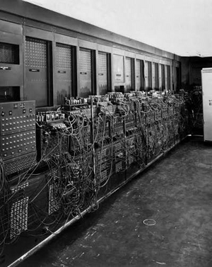
ENIAC (1946): Built to calculate artillery firing tables, it was one of the earliest fully electronic, general-purpose digital computers.ENIAC
Physical Specifications and Computing Capabilities of the ENIAC (1946)
20 accumulators (storing ten 10-digit decimal numbers each)
UNIVAC I (1951): The first commercially produced digital computer designed for business and administrative applications.
UNIVAC I
Physical Specifications and Computing Capabilities of the UNIVAC I (1951)
Category
Characteristic
Details
Physical Specifications
Floor Space
~35.5 m²
Weight
~13 tons
Power Draw
~125 kW
Internal Components
~5,200 vacuum tubes, 18,000 crystal diodes
Primary Storage
Mercury delay line memory (1,000 words of 12 decimal characters each)
Computing Capabilities
Addition / Subtraction
~1,905 operations per second
Multiplication
~455 operations per second
Division
~257 operations per second
Clock Speed
2.25 MHz
Input / Output Method
Unityper (magnetic tape units), punched card converter, electric typewriter
The Von Neumann Architecture (1945–1946)
Formulated by mathematician John von Neumann, this theoretical framework defines the core hardware layout used by modern computers, including PCs, smartphones, and embedded systems.
Core Components
The Von Neumann model divides a computer system into four main functional blocks connected by buses:
Central Processing Unit (CPU) : The brain of the computer that processes all data.
Control Unit (CU): Fetches, decodes, and sequences instructions from memory.
Arithmetic Logic Unit (ALU): Executes mathematical calculations (`+`, `-`, `*`, `/`), logical operations (`AND`, `OR`), and comparisons (`<`, `>`, `=`).
Registers: High-speed temporary storage cells within the CPU core.
Main Memory (RAM): Volatile storage holding the current program instructions and active data.
Input/Output (I/O) Unit: Interfaces with external peripherals (e.g., keyboards, displays).
System Buses: Communication pathways that transmit data, memory addresses, and control signals.
Era III: Second and Third Generations (1958–1974)
The middle of the 20th century saw massive strides in miniaturization, execution speed, and software capability. Computing transitioned from room-sized vacuum tube machines to more reliable, solid-state systems.
Second generation: The transistor era (1958–1964)
In 1958, transistors replaced delicate vacuum tubes as the fundamental switching component in computers.
Hardware advances: Transistors made computers significantly smaller, cheaper, faster, and far more energy-efficient. Data storage shifted toward magnetic tapes and magnetic drums.
Software revolution: Programmers moved away from raw machine code. This era marked the birth of early high-level programming languages:
FORTRAN: Developed for complex scientific and mathematical calculations.
COBOL: Created for business, finance, and administrative processing systems.
ALGOL: Designed for algorithmic and scientific computations.
Third generation: Integrated circuits (1964–1974)
The third generation was defined by the invention of the Integrated Circuit (IC), where multiple electronic components were combined onto a single silicon semiconductor chip.
Performance boost: ICs dramatically reduced energy consumption and physical footprint while increasing clock speeds and processing capacity.
Storage advances: Magnetic disk storage emerged, allowing faster, random access to data compared to sequential magnetic tapes.
Expanded software: Advanced operating systems and application software proliferated, enabling computer-aided design (CAD) and database management systems (DBMS).
Era IV: Fourth Generation & Modern Computing (1974–Present)
The fourth generation of computing is defined by the development of the microprocessor, which integrated the entire Central Processing Unit (CPU) onto a single integrated circuit chip.
The microprocessor & The PC revolution
Integrating all CPU components onto a single chip drastically reduced production costs and physical size while boosting processing speeds.
Personal computers (PCs): In 1981, IBM introduced the IBM PC, bringing computing power out of specialized laboratories and into homes and offices.
Storage advances: Internal hard disk drives (HDDs), floppy disks, and later solid-state drives (SSDs) expanded local data storage capacity.
Network integration: Devices became interconnected through local networks and the Internet, expanding access to information.
Modern architecture enhancements
Modern processors expand upon the classical Von Neumann model to overcome performance bottlenecks and execute instructions faster:
Floating-Point Unit (FPU): A specialized hardware block designed specifically to handle fractional, trigonometric, and logarithmic operations in a single cycle.
Cache memory (L1, L2, L3): High-speed internal memory layers that store frequently accessed data close to the CPU core to reduce memory latency.
System buses:
Front-Side Bus (FSB): Connects the secondary cache and CPU to the motherboard and main memory (typically 64 bits wide).
Back-Side Bus (BSB): High-speed internal interface connecting the CPU core directly to L1 and L2 caches.
Parallelism & Specialization: Advanced techniques such as instruction pipelining, superscalar execution, hyper-threading, multi-core architectures, and specialized instruction sets (MMX, SSE) allow computers to process multiple instructions simultaneously.
Comparison of computing generations, key technologies, and physical specifications
Era / Generation
Years
Key Technological Aspects
Representative Computer & Physical Specifications
Pre-Generation ⚙️
1833–1944
Transition from mechanical to electro-mechanical computing.
Introduction of foundational units: Input, Memory (Store), Control Unit, ALU (Mill), Output.
Implementation of punched cards for data input.
IBM Harvard Mark I (1944)
Dimensions: 17 m long × 2 m high
Weight: 70 tons
Components: 700,000 moving parts
Speed: Addition < 1s, Multiplication ~6s
1st Generation 💡
1946–1958
Built using vacuum tubes.
Large physical footprint, high power draw, complex maintenance.