Hardware history
Template:Infobox historic computing technology
Overview
The transition from manual calculation to automated computing began with 19th-century mechanical designs and culminated in mid-20th-century electro-mechanical systems.
Era I: Mechanical pioneers (1833)
Charles Babbage and the Analytical Engine
In 1833, British mathematician Charles Babbage conceived the Analytical Engine, widely considered the theoretical precursor to the modern general-purpose electronic computer. Although never fully constructed during his lifetime due to mechanical limitations, Babbage's design established five core functional units:
- Input devices 📥: For entering instructions and data.
- Memory 🧠: For holding numbers and intermediate results.
- Control Unit 🎛️: For directing the sequence of operations.
- Arithmetic Logic Unit (The Mill) 🔢: For executing mathematical calculations.
- Output Devices 📤: For displaying or printing results.

More about Babbage analytic engine
The "Real" Analytical Engine (1833)
In 1833, Charles Babbage designed the Analytical Engine, widely considered the theoretical precursor to the modern general-purpose computer.
How it worked
The Analytical Engine was designed as a fully mechanical, steam-powered machine. Remarkably, its architecture mirrored the core components of modern computers long before electronics existed:
- Input system 📥: Instructions and data were fed into the machine using punched cards (a technique adapted from the Jacquard loom).
- The store (Memory) 🧠: A vast system of gears and counter wheels designed to hold up to 1,000 numbers of 50 decimal digits each.
- The Mill (ALU) 🔢: The mechanical processing unit capable of performing basic arithmetic (addition, subtraction, multiplication, division) and comparison tests.
- Control unit 🎛️: Barrel controllers (similar to those in music boxes) orchestrated operations, allowing for conditional branching ("if/then") and loops
- Output system 📤: Results were sent to a printer, a curve plotter, or punched directly onto cards.
Construction status
- During Babbage's lifetime: Babbage never completed a fully functional, full-scale Analytical Engine due to funding shortages, personal disputes, and the limits of 19th-century mechanical precision.
- Modern reconstructions: While a complete Analytical Engine has never been built, London's Science Museum constructed Babbage's simpler Difference Engine No. 2 in 1991, proving his mechanical theories were sound. An ongoing initiative called Plan 28 aims to construct a working Analytical Engine using Babbage's original drawings.

Ada Lovelace: The first programmer
Ada Lovelace (1815–1852), an English mathematician and writer, played a pivotal role in the conceptualization of general-purpose computing. While translated work on Babbage's Analytical Engine was published in 1842 by Italian engineer Luigi Menabrea, Lovelace added extensive "Notes" that were three times longer than the original paper itself.
Key contributions
- The first computer algorithm: In "Note G," Lovelace detailed a step-by-step method for calculating Bernoulli numbers using the Analytical Engine. This execution plan is widely recognized as the world's first published algorithm designed specifically for implementation on a computer.
- Beyond pure calculation: Lovelace had a visionary insight that set her apart from her contemporaries. While Babbage focused primarily on numerical calculation, Lovelace realized that if the machine could manipulate symbols representing any entity (such as musical notes or text), it could manipulate non-numeric data[cite: 1]. She famously suggested that the engine "might compose elaborate and scientific pieces of music of any degree of complexity or extent."
- Foundational programming concepts: Her notes introduced early conceptual models of programming techniques still used today, including loops, subroutines, and conditional instruction execution.
Electro-mechanical realization (1944)
The IBM Harvard Mark I
In 1944, Howard Aiken realized Babbage's vision by completing the IBM Harvard Mark I. It was the first fully functional, large-scale electro-mechanical computer.

| Feature | Specification |
|---|---|
| Dimensions | 17 meters long × 2 meters high |
| Weight | Approximately 70 tons |
| Components | 700,000 moving parts; hundreds of kilometers of wiring |
| Input Method | 80-column IBM punched cards |
| Performance | Addition: < 1 second; Multiplication: ~6 seconds |
Era II: First-generation electronic computers (1946–1958)
The first generation of electronic computing replaced electro-mechanical switches with vacuum tubes. While this drastically increased processing speed, these early computers had a massive physical footprint, consumed enormous amounts of electricity, and required frequent maintenance due to tube failure.
Key early systems
- ENIAC (1946): Built to calculate artillery firing tables, it was one of the earliest fully electronic, general-purpose digital computers.
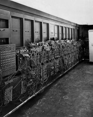
ENIAC

| Category | Characteristic | Details |
|---|---|---|
| Physical Specifications | Floor Space | ~167 m² |
| Weight | ~30 tons | |
| Dimensions | ~2.4 m × 0.9 m × 30.5 m | |
| Power Draw | ~150 kW to 160 kW | |
| Internal Components | ~17,468 vacuum tubes, 7,200 diodes, 70,000 resistors, 10,000 capacitors | |
| Computing Capabilities | Addition / Subtraction | 5,000 operations per second |
| Multiplication | ~357 operations per second | |
| Division / Square Root | ~35 operations per second | |
| Clock Speed | 100 kHz (100,000 cycles per second) | |
| Memory / Storage | 20 accumulators (storing ten 10-digit decimal numbers each) |
- UNIVAC I (1951): The first commercially produced digital computer designed for business and administrative applications.

| Category | Characteristic | Details |
|---|---|---|
| Physical Specifications | Floor Space | ~35.5 m² |
| Weight | ~13 tons | |
| Power Draw | ~125 kW | |
| Internal Components | ~5,200 vacuum tubes, 18,000 crystal diodes | |
| Primary Storage | Mercury delay line memory (1,000 words of 12 decimal characters each) | |
| Computing Capabilities | Addition / Subtraction | ~1,905 operations per second |
| Multiplication | ~455 operations per second | |
| Division | ~257 operations per second | |
| Clock Speed | 2.25 MHz | |
| Input / Output Method | Unityper (magnetic tape units), punched card converter, electric typewriter |
The Von Neumann Architecture (1945–1946)
Formulated by mathematician John von Neumann, this theoretical framework defines the core hardware layout used by modern computers, including PCs, smartphones, and embedded systems.
Core Components
The Von Neumann model divides a computer system into four main functional blocks connected by buses:
- Central Processing Unit (CPU) : The brain of the computer that processes all data.
- Control Unit (CU): Fetches, decodes, and sequences instructions from memory.
- Arithmetic Logic Unit (ALU): Executes mathematical calculations (`+`, `-`, `*`, `/`), logical operations (`AND`, `OR`), and comparisons (`<`, `>`, `=`).
- Registers: High-speed temporary storage cells within the CPU core.
- Main Memory (RAM): Volatile storage holding the current program instructions and active data.
- Input/Output (I/O) Unit: Interfaces with external peripherals (e.g., keyboards, displays).
- System Buses: Communication pathways that transmit data, memory addresses, and control signals.
Era III: Second and Third Generations (1958–1974)
The middle of the 20th century saw massive strides in miniaturization, execution speed, and software capability. Computing transitioned from room-sized vacuum tube machines to more reliable, solid-state systems.
Second generation: The transistor era (1958–1964)
In 1958, transistors replaced delicate vacuum tubes as the fundamental switching component in computers.
- Hardware advances: Transistors made computers significantly smaller, cheaper, faster, and far more energy-efficient. Data storage shifted toward magnetic tapes and magnetic drums.
- Software revolution: Programmers moved away from raw machine code. This era marked the birth of early high-level programming languages:
- FORTRAN: Developed for complex scientific and mathematical calculations.
- COBOL: Created for business, finance, and administrative processing systems.
- ALGOL: Designed for algorithmic and scientific computations.
Third generation: Integrated circuits (1964–1974)
The third generation was defined by the invention of the Integrated Circuit (IC), where multiple electronic components were combined onto a single silicon semiconductor chip.
- Performance boost: ICs dramatically reduced energy consumption and physical footprint while increasing clock speeds and processing capacity.
- Storage advances: Magnetic disk storage emerged, allowing faster, random access to data compared to sequential magnetic tapes.
- Expanded software: Advanced operating systems and application software proliferated, enabling computer-aided design (CAD) and database management systems (DBMS).
Era IV: Fourth Generation & Modern Computing (1974–Present)
The fourth generation of computing is defined by the development of the microprocessor, which integrated the entire Central Processing Unit (CPU) onto a single integrated circuit chip.
The microprocessor & The PC revolution
Integrating all CPU components onto a single chip drastically reduced production costs and physical size while boosting processing speeds.
- Personal computers (PCs): In 1981, IBM introduced the IBM PC, bringing computing power out of specialized laboratories and into homes and offices.
- Storage advances: Internal hard disk drives (HDDs), floppy disks, and later solid-state drives (SSDs) expanded local data storage capacity.
- Network integration: Devices became interconnected through local networks and the Internet, expanding access to information.
Modern architecture enhancements
Modern processors expand upon the classical Von Neumann model to overcome performance bottlenecks and execute instructions faster:
- Floating-Point Unit (FPU): A specialized hardware block designed specifically to handle fractional, trigonometric, and logarithmic operations in a single cycle.
- Cache memory (L1, L2, L3): High-speed internal memory layers that store frequently accessed data close to the CPU core to reduce memory latency.
- System buses:
- Front-Side Bus (FSB): Connects the secondary cache and CPU to the motherboard and main memory (typically 64 bits wide).
- Back-Side Bus (BSB): High-speed internal interface connecting the CPU core directly to L1 and L2 caches.
- Parallelism & Specialization: Advanced techniques such as instruction pipelining, superscalar execution, hyper-threading, multi-core architectures, and specialized instruction sets (MMX, SSE) allow computers to process multiple instructions simultaneously.
Comparison of computing generations, key technologies, and physical specifications
| Era / Generation | Years | Key Technological Aspects | Representative Computer & Physical Specifications |
|---|---|---|---|
| Pre-Generation ⚙️ | 1833–1944 |
|
IBM Harvard Mark I (1944)
|
| 1st Generation 💡 | 1946–1958 |
|
ENIAC (1946) & UNIVAC I (1951)
|
| 2nd Generation ⚡ | 1958–1964 |
|
Transistorized room-sized mainframe systems utilizing magnetic drum and tape storage. |
| 3rd Generation 🔲 | 1964–1974 |
|
Mainframes and minicomputers integrated onto single-chip component boards. |
| 4th Generation 🔬 | 1974–Present |
|
IBM PC (1981) & Modern Microprocessors
|
